A Gentle Introduction of Linear Mixed-Effects Models to Neuroscientists
Part I. Why do the conventional methods fail in the presence of correlated data?
Clustered data are probably the norm rather than the exception in neuroscience research. As a result, the observations often correlated, which can lead to incorrect statistical inference if not analyzed appropriately.

To see this, we are going to assess the degree of data dependency in our motivating example (Example 1). We will use this example to understand the dependence due to clustering (animal effects) and what is the consequence of ignoring the dependence structure. The software we will use is R, which is a free and open source software (CRAN). One major advantage of R over other open source or commercial software is that R is verified and has a rich collection of user-contributed packages (over 15,000), greatly facilitating a programing environment for developers and access to cutting-edge statistical methods. Among the numerous packages that can fit LME and GLMM, we suggest the readers start with the following R packages: lme4, nlme, icc, and pbkrtest. If they have not been installed into your computer, you need to install them
We quantify the magnitude of data dependence in this example, we computed the intra-class correlation (ICC) for each condition. In this example, the ICC is the ratio of between-animal variance to the total variance. Its range is typically between 0 and 1, the closer it is to 1, the more similar the observations within the same animal. Use the code below to generate 1000 data sets, each of which follows the same ICC structure and assumes NO difference between the five conditions. Surprisingly, the type I error rate when treating 1200 neurons as independent observations is over 90% at the significance level of α=0.05.
Next, we import the data to R and analyze its intra-class correlation (ICC). In this example, we measured the change in pCREB immunoreactivity of non-PV, 1,200 putative excitatory neurons in visual cortex layer 2/3 at different time points: collected at baseline, 24, 48, 72 hours, and 1 week following ketamine treatment, collected from 24 mice. See Grieco et al. (2020) for more details. The following figure shows the change in pCREB immunoreactivity tend to be clustered, i.e., measurements from the same animal tend to more similar to each other than measurements from different animals.
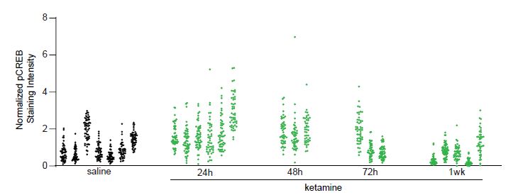
Thus, the 1,200 neurons should not be treated as 1,200 independent neurons. We quantify the magnitude of data dependence in this example, we computed the ICC for each condition. In this example, the ICC is the ratio of between-animal variance to the total variance. Its range is typically between 0 and 1, the closer it is to 1, the more similar the observations within the same animal.
The results are organized in the following Table:
| Saline (7 mice) | 24h (6 mice) | 48h (3 mice) | 72h (3 mice) | 1wk (5 mice) | |
|---|---|---|---|---|---|
| # of cells | 357 | 209 | 139 | 150 | 245 |
| ICC | 0.61 | 0.33 | 0.02 | 0.63 | 0.54 |
When dependence is not adequately accounted for, the type I error rate can be much higher than the significance level. To see how serious the problem is, we examine the false positives based on the dependence structure observed in our own study. Use the code below to generate 1000 data sets, each of which follows the same ICC structure and assumes NO difference between the five conditions. Surprisingly, the type I error rate when treating 1,200 neurons as independent observations is over 90% at the significance level of α=0.05.
The ICC, design effect, and effective sample sizes (Table *) indicate that the dependency due to clustering is substantial. Therefore, the 1,200 neurons should not be treated as 1,200 independent cells. This is a situation for which the number of observational units is much larger than the number of experimental units. We will show how to use a linear mixed-effects model to analyze the data in the next section.
Part II: Examples of Mixed-effects models
(a) Conduct LME in R
NLME and LME4 are the two most popular R packages for LME analysis. Besides the use of slightly different syntaxes for random effects, lme (NLME) and lmer (LME4) do differ in several other ways, such as flexibility in modeling the types of outcomes, how they handle heteroscedasticity, the covariance structure of random effects, crossed random effects, and their approximations for test statistics. A full description of these differences is beyond the scope of this article. We refer the interested readers instead to the references.
A practical issue of the lmer function is that although it provides point estimates and standard errors, it does not generate p-values. This is because the exact null distributions of t or F statistics are not known, as explained in Baayen et al. (2008). Extensions to LME4 have been developed to compute p values by either approximation methods (e.g., R pcakge lmerTest) or resampling methods such as Bootstrap (R package pbkrtest). R code with detailed comments for all the three examples is available in the supplementary materials.
Example 1. The data have been described in Part I. We used an LME with an animal-specific random-effects to handle the dependency due to clustering. As a comparison, we also run the LM model, which erroneously pools all the neurons together and treats them as independent data points. The significance levels of the LM p-values are much higher (p-values: 0.0084 v.s. 2.2×10⁻¹⁶). However, remember that the LM analysis should not be used because, as shown in Part I, its type I error rate is unacceptably high.
Example 2. Data were derived from an experiment to determine how in vivo calcium (Ca++) activity of PV cells (measured longitudinally by the genetically encoded Ca++ indicator GCaMP6s) changes over time after ketamine treatment 13. We show four mice whose Ca++ event frequencies were measured at 24h, 48h, 72h, and 1 week after ketamine treatment and compare Ca++ event frequency at 24h to the other three time points. In total, Ca++ event frequencies of 1,724 neurons were measured. First let’s evaluate the effect of ketamine using LM (or ANOVA, which ignores mouse-specific effect).
The LM (or ANOVA, t-test) analysis results indicate significantly reduced Ca++ activity at 48h relative to 24h with p=4.8×10⁻⁶, and significantly increased Ca++ event frequency at 1wk compared to 24h with p=2.4×10⁻³. However, if we account for repeated measures due to cells clustered in mice using LME, all the p-values are greater than 0.05
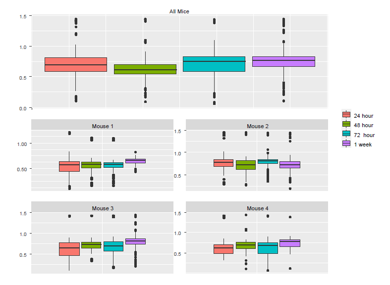
The last column of the table above shows that Mouse 2 contributed 43% cells, which might explain why the pooled data are more similar to Mouse 2 than to the other mice. The lesson from this example is that naively pooling data from different animals is a potentially dangerous practice, as the results can be dominated by a single animal that can misrepresent a substantial proportion of the measured data. Investigators limited to using LM often notice outlier data of a single animal and they may agonize whether they are justified in “tossing that animal” from their analysis, sometimes by applying “overly creative post-hoc exclusion criteria”. The other way out of this thorny problem is the brute force approach of repeating the experiment with a much larger sample size – a more honest, but expensive solution. Application of LME solves this troubling potential problem as it takes dependency and weighting into account
| 48h | 72h | 1wk | |
|---|---|---|---|
| LM est | -0.078±0.017 | 0.009±0.017 | 0.050±0.016 |
| LM p | 4.8×10⁻⁶ | 0.595 | 2.4×10⁻³ |
| LME est | -0.017±0.017 | 0.009±0.017 | 0.029±0.016 |
| LME p | 0.325 | 0.574 | 0.079 |
To understand the discrepancy between the results from LM and LME, we created boxplots using individual mice as well as all the mice (Figure *). Although the pooled data (Figure *a) and the corresponding p-value from the LM show significant reduction in Ca++ activities from 24h to 48h, we noticed that the only mouse showing a noticeable reduction was Mouse 2. In fact, close examination of Figure 4b suggests that there might be small increases in the other three mice. To examine why the pooled data follow the pattern of Mouse 2 and not that of other mice, we checked the number of neurons in each of the mouse-by-time combinations
In this example, the number of levels in the random-effects variable is four, as there are four mice. This number may be smaller than the recommended number for using random-effects. However, as discussed in Gelman and Hill (2007), using a random-effects model in this situation of a small sample size might not do much harm. An alternative is to include the animal ID variable as a factor with fixed animal effects in the conventional linear regression. Note that neither of the two analyses is the same as fitting a linear model to the pooled cells together, which erroneously ignores the between-animal heterogeneity and fails to account for the data dependency due to the within-animal similarity. In a more extreme case, for an experiment using only two monkeys, naively pooling the neurons from the two animals faces the risk of making conclusions mainly from one animal and unrealistic homogeneous assumptions across animals, as discussed above. A more appropriate approach is to analyze the animals separately and check whether the results from these two animals “replicate” each other. Exploratory analysis such as data visualization is highly recommended to identify potential issues.
Example 3. Cells are nested in animals. The best practice is to code cell ID uniquely. See GLMM FQA. In this experiment, Ca++ event integrated amplitudes are compared between baseline and 24h after ketamine treatment 13. 622 cells were sampled from 11 mice and each cell was measured twice (baseline and after ketamine treatment). As a result, correlation arises from both cells and animals, which creates a three-level structure: measurements within cells and cells within animals. It is clear that the ketamine treatment should be treated as a fixed effect. The choice for random effects deserves more careful consideration. The hierarchical structure, i.e., two observations per cell and multiple cells per animal suggests that the random effects of cells should be nested within individual mice. By including the cell variable in the random effect, we implicitly use the change from “before” to “after” treatment for each cell. This is similar to how paired data are handled in a paired t-test. Moreover, by specifying that the cells are nested within individual mice, we essentially model the correlations for both mouse and cell levels
For the treatment effect, LME and LM produce similar estimates; however, the standard error of the LM was larger. As a result, the p-value based on LME was smaller (0.0036 for LM vs 0.0001 for LME). In this example, since the two measures from each cell are positively correlated (Figure *a), the variance of the differences is smaller than the variance of baseline or after treatment (Figure *b). As a result, the more rigorous practice of using cell effects as random effects leads to a lower p-value for Example 3.
A note on “nested” random effects. When specifying the nested random effects by using “random =~1| midx/cidx”. This leads to random effects of two levels: the mouse level and the cells-within-mouse level. This is specification is important if same cell IDs might appear in different mice. When each cell has a unique ID, just like “cidx” variable in Example 3, it does not matter and “random =list(midx=~1, cidx=~1)” leads to exactly the same model.

(B) Conduct GLMM in R
The computation involved in GLMM more much challenging. The “glmer” function in the lme4 package can be used to fit a GLMM, which will be shown in Example 4.
Example 4. In the previous examples, the outcomes of interest are continuous. In particular, some of them were transformed from original measures so that the distribution of the outcome variable has a rough bell shape. In many situations, the outcome variable we are interested has a distribution that far away from normal. Consider a simulated data set based upon part of the data used in Wei et al 2020. In our simulated data, a tactile delayed response task, eight mice were trained to use their whiskers to predict the location (left or right) of a water pole and report it with directional licking (lick left or lick right). The behavioral outcome we are interested in is whether the animals made the correct predictions. Therefore, we code correctly lick left or lick right as 1 and erroneously lick left or lick right as 0. In total, 512 trials were generated, which include 216 correct trials and 296 wrong trials. One question we would like to answer is whether a particular neuron is associated with prediction. More specifically, we would like to demonstrate the usage of GLMM by analyzing the prediction outcome and mean neural activity levels (measured by dF/F) from the 512 trials. The importance of modeling correlated by introducing random effects has been demonstrated in the previous examples. In this example, we focus on how to interpret results from a GLMM model in the waterlick experiment
Like a GLM, a GLMM requires the specification of a family of the distributions of the outcomes and an appropriate link function. Because the outcomes in this example are binary, the natural choice, which is often called the canonical link of the “binomial” family, is the logistic link. For each family of distributions, there is a canonical link, which is well defined and natural to that distribution family. For example, the canonical link for a Gaussian (Normal) and Binomial distributed random variable is the identity link and the logistic link, respectively. For researchers with limited experience with GLM or GLMM, a good starting point, which is often a reasonable choice, is to use the default choice (i.e., the canonical link). We refer readers curious about non-canonical link functions to Czadoy and Munk (2000)
The default method of parameter estimation is the maximum likelihood with Laplace approximation. In many studies, the coefficient of a particular independent variable is of the primary interest. As shown in the Fixed effects section, the estimate of the dF/F is 0.06235, the standard error is 0.01986, and the reported p-value (which is based on the large-sample Wald test) is 0.01693. In a logistic regression, the estimated coefficient of an independent variable is typically interpreted using the percentage of odds changed for a one unit increase in the independent variable. In this example, exp(0.06235)=1.06, indicating that 6% increase in making the correct prediction with a one unit increase in dF/F. Similarly, we can construct a 95% C.I., which is [2%-11%]
An alternative way to compute a p-value is to use a likelihood ratio test by comparing the likelihoods of the current model and a reduced model.
In the output, the “Chisq” is the -2*log(L0/L1), where L1 is the maximized likelihood of the model with dff and L0 is the maximized likelihood of the model without the pff. The p-value 0.001568 was obtained using the large-sample likelihood ratio test
In GLMM, the p-value based on large-sample approximations might not be accurate. It is helpful to check whether nonparametric tests lead to similar findings. For example, one can use a parametric bootstrap method (Halekoh, Højsgaard 2014). For this example, the p-value from the parametric bootstrap test, which is slightly less significant than the p-values from the Wald or LRT test
This procedure takes longer than fitting a single model, as 1000 (the default) samples were generated to understand the null distribution of the likelihood ratio statistic. One way to expediate the computation is by using multiple cores. We encourage the interested readers to read the documentation of this package, which is available at https://cran.r-project.org/web/packages/pbkrtest/pbkrtest.pdf
References:
Ulrich Halekoh, Søren Højsgaard (2014). A Kenward-Roger Approximation and Parametric Bootstrap Methods for Tests in Linear Mixed Models – The R Package pbkrtest., Journal of Statistical Software, 58(10), 1-30., https://www.jstatsoft.org/v59/i09/