Zhaoxia Yu#, Michele Guindani, Steven F. Grieco, Lujia Chen, Todd C. Holmes, Xiangmin Xu#
(2021) Neuron https://doi.org/10.1016/j.neuron.2021.10.030
1.Supplemental data download
2.Online version of our additional materials
See our COLAB version of interactive codes :
Supplemental Information
(1) Why do the conventional methods fail in the presence of correlated data?
In basic neuroscience research, data dependency due to clustering or repeated measurements is probably the norm rather than the exception. Unfortunately, the most widely used methods under these situations are still the t-test and ANOVA, which do not take dependence into account, thus leading to incorrect statistical inference and misleading conclusions.
We will use a data set collected from our own work to assess the degree of data dependency due to clustering (animal effects) and to illustrate the consequences of ignoring the dependent structure. In this example, we measured the change in pCREB immunoreactivity of 1,200 putative excitatory neurons in mouse visual cortex at different time points: collected at baseline (saline), 24, 48, 72 hours, and 1 week following ketamine treatment, from 24 mice. See Grieco et al. (2020) for more details. Figure S1 shows that the changes in pCREB immunoreactivity tend to be clustered, i.e., measurements from the same animal tend to be more similar to each other than measurements from different animals.
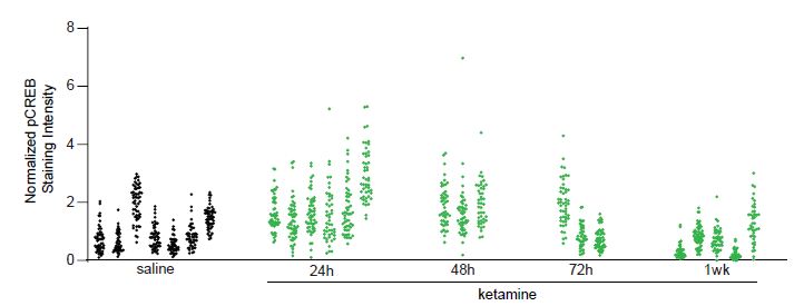
Figure S1: Normalized pCREB staining intensity values from 1,200 neurons (Example 1). The values in
each cluster were from one animal. In total, pCREB values were measured for 1,200 neurons from 24
mice at five conditions: saline (7 mice), 24h (6 mice), 48h (3 mice), 72h (3 mice), 1week (5 mice) after
treatment.
We compute the intra-class correlation (ICC) to quantify the magnitude of dependency within animals using the software R, a free and open source software (CRAN) (R Development Core Team, 2020). One major advantage of R over other open source or commercial software is that R is widely adopted and continuously reassessed for accuracy, and has a rich collection of user-contributed packages (over 15,000), thus supporting a programing environment for developers and access to cutting-edge statistical methods. In this tutorial, we will use the following R packages: lme4 (Bates et al., 2014), nlme (Pinheiro et al., 2007), icc (Wolak and Wolak, 2015), pbkrtest (Halekoh and Højsgaard, 2014), brms (Bürkner, 2017; Bürkner, 2018), lmerTest (Kuznetsova et al., 2017), emmeans (Lenth et al., 2019), car (Fox and Weisberg, 2018) , and sjPlot (Lüdecke, 2018). If they have not been installed onto your computer, you will need to install them by removing the “#” symbol and copy one line at a time to your R console. The “#” symbol is used for commenting out code in R. The installation of a package to a computer only needs to be done once. However, the libraries for data analysis need to be loaded each time you start the R software. We recommend you only load a library when it is needed.
install.packages("lme4")
install.packages("nlme")
install.packages("ICC")
install.packages("brms")
install.packages("pbkrtest")
install.packages("emmeans")
install.packages("car")
install.packages("sjPlot")
We start with reading the pCREB data (Example 1) into R. Because the data file is comma separated, we use the function “read.csv” to read it. The option “head=T” reads the first row as the column names. Most R packages of LME require the “long”, also known as “vertical” format, in which data
are organized in a rectangular data matrix, i.e., each row of the dataset contains only the values for one observation. The columns contain necessary information about this observation such as the experimental condition, treatment, cell ID, and animal ID. In this example, the data are stored in a 1,200-by-3 matrix, with the first column being the pCREB immunoreactivity values, the second column being the treatment labels, and the last column being the animal identification numbers. The treatment information is in the second column and it is coded as labels 1 through 5: 1 for baseline (saline), 2-5 for 24, 48, 72 hours, and 1 week after ketamine treatment, respectively. By default, the treatment information is read into numerical values. To convert it to a categorical variable, we apply the “as.factor” function to the treatment variable.
# The following lines of code read the Example 1 data
Ex1 = read.csv("Example1.txt", head=T)

# checking the dimensions of the dataset
dim(Ex1)

# checking the names of each column
names(Ex1)

# a frequency table for the treatment variable
table(Ex1$treatment_idx)

# a frequency table for the measurements in each mouse
table(Ex1$midx)

#Do not forget to factor the treatment IDs
Ex1$treatment_idx = as.factor(Ex1$treatment_idx)
Next, we examine the magnitude of clustering due to animal effects by computing the ICC for each treatment group.
### load the ICC library
library(ICC) #load the library to conduct ICC analysis with its function ICCbare

### conduct ICC analysis by organizing all the information into a data frame
icc.analysis=data.frame(n=rep(0,5), icc=rep(0,5), design.effect=rep(0,5),
effective.n=rep(0,5), M=rep(0,5), cells=rep(0,5))

for(i in 1:5){
    trt= Ex1[Ex1$treatment_idx==i,]
    trt$midx=factor(trt$midx)
    icc=ICCbare(factor(trt$midx), trt$res) #ICCbare is a function in the ICC package
    icc.analysis$cells[i]=dim(trt)[1]
    M=dim(trt)[1]/length(unique( trt$midx))
    def=1 + icc*(M-1)
    icc.analysis$n[i]=length(unique( trt$midx))
    icc.analysis$icc[i]=icc
    icc.analysis$design.effect[i]=def
    icc.analysis$effective.n[i]=dim(trt)[1]/def
    icc.analysis$M[i]=M
}
icc.analysis

n icc design.effect effective.n M cells
1 7 0.62094868 32.047434 11.139737 51.00000 357
2 6 0.33006327 17.668195 17.489053 51.50000 309
3 3 0.01780304 1.807071 76.920039 46.33333 139
4 3 0.62810904 31.777343 4.720344 50.00000 150
5 5 0.53694579 26.773398 9.150874 49.00000 245
The results are organized in the following table:
| Saline (7 mice) | 24h (6 mice) | 48h (3 mice) | 72h (3 mice) | 1wk (5 mice) | ||
| # of cells | 357 | 209 | 139 | 150 | 245 | |
| ICC | 0.61 | 0.33 | 0.02 | 0.63 | 0.54 |
The ICC indicates that the dependency due to clustering is substantial. Therefore, the 1,200 neurons should not be treated as 1,200 independent cells. When dependence is not adequately accounted for, the type I error rate can be much higher than the pre-chosen level of significance. To see how serious this problem is, we examine the false positives based on the dependence structure observed in our own study. In the simulation script we wrote “simulation_TypeIErrorRate.R” (see download section above), we generated 1000 data sets, each of which follows the same ICC structure and assumes NO difference between the five conditions. Surprisingly, the type I error rate when treating 1,200 neurons as independent observations is over 90% at the significance level of α=0.05.
### run the simulation script
source("simulation_TypeIErrorRate.R")
[1] "Type I error rate of LM at significance level 0.05: "
[1] 0.9
[1] "Type I error rate of LME at significance level 0.05: "
[1] 0.086
This is a situation for which the number of observational units is much larger than the number of experimental units. We will show how to use a linear mixed-effects model to correctly analyze the data in the next section.
(2) Mixed-effects model analysis
The word “mixed” in linear mixed-effects (LME) means that the model consists of both fixed and random effects. Fixed effects refer to fixed but unknown coefficients for the variables of interest and explanatory covariates, as identified in the traditional linear model (LM). Random effects, refer to variables that are not of direct interest – however, they may potentially lead to correlated outcomes. A major difference between fixed and random effects is that the fixed effects are considered as parameters whereas the random effects are considered as random variables drawn from a distribution (e.g., a normal distribution).
In order to apply the LME, it is necessary to understand its inner workings in sufficient detail. Let Yij indicate the jth observation of the ith mouse, , and (xij,1, …, xij,4) be the dummy variables for the treatment labels with xij,1 = 1 for 24 hours, xij,2 = 2 for 48 hours, xij,3 = 3 for 72 hours, and xij,4 = 4 for 1 week after ketamine treatments, respectively. Remarks. (1) Note that the variable for baseline xij,0 = 0 is not needed in the equation, as the effect at baseline serves as the reference for other groups. (2) In the data we used levels 1-5 instead of 0-4. Because treatment labels are categorical variables, there is no difference between using 1-5 and 0-4 as labels.
Because there are multiple observations from the same animal, the data are naturally clustered by animal. We account for the resulting dependence by adding an animal specific mean to the regression framework discussed in the previous section, as follows:
Yij = β0 + xij,1β1 + … + xij,4β4 + ui + Ԑij, i=1, …, 24; j=1, …, ni;
where ni is the number of observations from the ith mouse, ui indicates the deviance between the overall intercept β0 and the mean specific to the ith mouse, and Ԑij represents the deviation in pCREB immunoreactivity of observation (cell) j in mouse i from the mean pCREB immunoreactivity of mouse i. Among the coefficients, the coefficients of the fixed-effects component, (β0, β1, β2, β3, β4), are assumed to be fixed but unknown, whereas (u1, …, u24) are treated as independent and identically distributed random variables from a normal distribution with mean 0 and a variance parameter that reflects the variation across animals. It is important to notice that the cluster/animal-specific means are more generally referred to as random intercepts in an LME. Equivalently, one could write the previous equation by using a vector (zij,1, …, zij,24) of dummy variables for the cluster/animal memberships such that zij, k=1 for i=k and 0 otherwise:
Yij = β0 + xij,1β1 + … + xij,4β4 + zij,1u1 + … + zij,24u24 + Ԑij, i=1, …, 24; j=1, …, ni;
In the model above, Yij is modeled by four components: the overall intercept β0, which is the population mean of the reference group in this example, the fixed-effects from the covariates (xij,1, …, xij,4), the random-effects due to the clustering (zij,1, …, zij,24), and the random errors Ԑij’s, assumed to be i.i.d. from a normal distribution with mean 0.
It is often convenient to write the LME in a very general matrix form, which was first derived in (Henderson et al., 1959). This format gives a compact expression of the linear mixed-effects model:
Y= β0 + Xβ +Zu + Ԑ,
where Y is an n-by-1 vector of individual observations, 1 is the n-by-1 vector of ones, the columns of X are predictors whose coefficients β, a p-by-1 vector, are assumed to be fixed but unknown, the columns of Z are the variables whose coefficients u, a q-by-1 vector, are random variables drawn from a distribution with mean 0 and a partially or completely unknown covariance matrix, and Ԑ is the residual random error.
Conduct LME in R
nlme and lme4 are the two most popular R packages for LME analysis. Besides the use of slightly different syntaxes for random effects, their main functions do differ in several other ways, such as their flexibility for modeling different types of outcomes, how they handle heteroscedasticity, the covariance structure of random effects, crossed random effects, and their approximations for test statistics. A full description of these differences is beyond the scope of this article. We refer interested readers instead to the documentation for each of the two packages. Next, we show how to analyze Examples 1-3 using linear mixed effects models.
Example 1. The data have been described in Part I. We first fit a conventional linear model using the lm function, which erroneously pools all the neurons together and treats them as independent observations.
################ Wrong analysis ####################
>#Wrong analysis: using the linear model
>obj.lm=lm(res~treatment_idx, data=Ex1)
>summary(obj.lm)
Call:
lm(formula = res ~ treatment_idx, data = Ex1)
S6
Residuals:
Min 1Q Median 3Q Max
-1.7076 -0.5283 -0.1801 0.3816 5.1378
Coefficients:
Estimate Std. Error t value Pr(>|t|)
(Intercept) 1.02619 0.03997 25.672 < 2e-16 ***
treatment_idx2 0.78286 0.05868 13.340 < 2e-16 ***
treatment_idx3 0.81353 0.07551 10.774 < 2e-16 ***
treatment_idx4 0.16058 0.07349 2.185 0.0291 *
treatment_idx5 -0.36047 0.06266 -5.753 1.11e-08 ***
---
Signif. codes: 0 ‘***’ 0.001 ‘**’ 0.01 ‘*’ 0.05 ‘.’ 0.1 ‘ ’ 1
Residual standard error: 0.7553 on 1195 degrees of freedom
Multiple R-squared: 0.2657, Adjusted R-squared: 0.2632
F-statistic: 108.1 on 4 and 1195 DF, p-value: < 2.2e-16

>summary(obj.lm)$coefficients
Estimate Std. Error t value Pr(>|t|)
(Intercept) 1.0261907 0.03997259 25.672363 4.064778e-116
treatment_idx2 0.7828564 0.05868406 13.340189 6.040147e-38
treatment_idx3 0.8135287 0.07550847 10.774006 6.760583e-26
treatment_idx4 0.1605790 0.07348870 2.185084 2.907634e-02
treatment_idx5 -0.3604732 0.06265813 -5.753015 1.112796e-08

>anova(obj.lm)
Analysis of Variance Table
Response: res
Df Sum Sq Mean Sq F value Pr(>F)
treatment_idx 4 246.62 61.656 108.09 < 2.2e-16 ***
Residuals 1195 681.65 0.570
---
Signif. codes: 0 ‘***’ 0.001 ‘**’ 0.01 ‘*’ 0.05 ‘.’ 0.1 ‘ ’ 1

>anova(obj.lm)[1,5]
[1] 1.17392e-78

>#wrong analysis: use ANOVA
>obj.aov=aov(res~treatment_idx, data=Ex1)
>summary(obj.aov)
Df Sum Sq Mean Sq F value Pr(>F)
treatment_idx 4 246.6 61.66 108.1 <2e-16 ***
Residuals 1195 681.6 0.57
---
Signif. codes: 0 ‘***’ 0.001 ‘**’ 0.01 ‘*’ 0.05 ‘.’ 0.1 ‘ ’ 1
In this example, the parameters of major interest are the coefficients of the treatments (1: baseline; 2: 24 hours; 3: 48 hours; 4: 72 hours; 5: 1 week following treatment). The summary function of the lm object provides the estimates, standard error, t statistics, and p-values for each time point after the treatment, with the before treatment measurement used as the reference. The overall significance of the treatment factor is performed using an F test, which is available in the ANOVA table by applying the anova function to the lm object. Equivalently, one can also use the aov function to obtain the same ANOVA table.
As explained in Part I, ignoring the dependency due to clustering can lead to unacceptably high type I error rates. We next fit a linear mixed effects model by including animal-specific means. This can be done using either nlme::lme (the lme function in the nlme package) or lme4::lmer (the lmer function in the lme4 package), as shown below
################## Linear Mixed-effects Model ###########################
> #use nlme::lme
> library(nlme) #load the nlme library
> # The nlme:lme function specifies the fixed effects in the formula
> # (first argument) of the function, and the random effects
> # as an optional argument (random=). The vertical bar | denotes that
> # the cluster is done through the animal id (midx)
> obj.lme=lme(res~treatment_idx, data= Ex1, random = ~ 1|midx)
> summary(obj.lme)

Linear mixed-effects model fit by REML
Data: Ex1
AIC BIC logLik
2278.466 2314.067 -1132.233
Random effects:
Formula: ~1 | midx
(Intercept) Residual
StdDev: 0.5127092 0.5995358
Fixed effects: res ~ treatment_idx
Value Std.Error DF t-value p-value
(Intercept) 1.0006729 0.1963782 1176 5.095642 0.0000
treatment_idx2 0.8194488 0.2890372 19 2.835098 0.0106
treatment_idx3 0.8429473 0.3588556 19 2.348988 0.0298
treatment_idx4 0.1898432 0.3586083 19 0.529389 0.6027
treatment_idx5 -0.3199877 0.3043369 19 -1.051426 0.3063
Correlation:
(Intr) trtm_2 trtm_3 trtm_4
treatment_idx2 -0.679
treatment_idx3 -0.547 0.372
treatment_idx4 -0.548 0.372 0.300
treatment_idx5 -0.645 0.438 0.353 0.353
Standardized Within-Group Residuals:
Min Q1 Med Q3 Max
-2.5388279 -0.5761356 -0.1128839 0.4721228 8.8600545
Number of Observations: 1200
Number of Groups: 24

>#use lme4::lmer
>library(lme4) #load the lme4 library

># The nlme:lme4 adds the random effects directly in the
># formula (first argument) of the function
>obj.lmer=lmer(res ~ treatment_idx+(1|midx), data=Ex1)
>summary(obj.lmer)

Linear mixed model fit by REML ['lmerMod']
Formula: res ~ treatment_idx + (1 | midx)
Data: Ex1
REML criterion at convergence: 2264.5
Scaled residuals:
Min 1Q Median 3Q Max
S8
-2.5388 -0.5761 -0.1129 0.4721 8.8601
Random effects:
Groups Name Variance Std.Dev.
midx (Intercept) 0.2629 0.5127
Residual 0.3594 0.5995
Number of obs: 1200, groups: midx, 24
Fixed effects:
Estimate Std. Error t value
(Intercept) 1.0007 0.1964 5.096
treatment_idx2 0.8194 0.2890 2.835
treatment_idx3 0.8429 0.3589 2.349
treatment_idx4 0.1898 0.3586 0.529
treatment_idx5 -0.3200 0.3043 -1.051
Correlation of Fixed Effects:
(Intr) trtm_2 trtm_3 trtm_4
tretmnt_dx2 -0.679
tretmnt_dx3 -0.547 0.372
tretmnt_dx4 -0.548 0.372 0.300
tretmnt_dx5 -0.645 0.438 0.353 0.353
On the method of parameter estimation for LME. Note that lme and lmer produce exactly the same coefficients, standard errors, and t statistics. By default, the lme and lmer function estimate parameters using a REML procedure. Estimation of the population parameters in LME is often conducted using maximum likelihood (ML) or REML, where REML stands for the restricted (or residual, or reduced) maximum likelihood. While the name REML sounds confusing, REML obtains unbiased estimators for the variances by accounting for the fact that some information from the data is used for estimating the fixed effects parameters. A helpful analogy is the estimation of the population variance by the maximum likelihood estimator Σi=1-n (𝑥𝑖 − 𝑥̅)2/𝑛, which is biased, or by an unbiased estimatorΣi=1-𝑛 (𝑥𝑖 − 𝑥̅)2/(𝑛-1). This strategy is helpful when n is small.
On the degrees of freedom and P-values. A noticeable difference between the lme and lmer outputs is that p-values are provided by lme but not lmer. The calculation of p-values in lme uses the degrees of freedom according to “the grouping level at which the term is estimated” (Pinheiro and Bates, 2006), which is the animal level in Example 1. However, the calculation of the degrees of freedom for a fixed model is not as straightforward as for a linear model (see the link here for some details). Several packages use more accurate approximations or bootstrap methods to improve the accuracy of p-values. In the following, we show different methods to compute (1) the overall p-value of the treatment factor, (2) pvalues for individual treatments, and (3) p-value adjustment for multiple comparisons. These p-values are for testing the fixed effects. We defer the discussion related to random effects until Example 3.
(1) The overall p-value for the treatment factor. This p-value aims to understand whether there is any statistically significant difference among a set of treatments. We offer several ways to calculate this type of p-values. When assessing the overall treatment effects using a likelihood ratio test, one should use maximum likelihood, rather than REML, when using lme or lmer.
> #overall p-value from lme
> Wald F-test from an lme object
> obj.lme=lme(res~treatment_idx, data= Ex1, random = ~ 1|midx)
> anova(obj.lme) #Wald F-test
numDF denDF F-value p-value
(Intercept) 1 1176 142.8589 <.0001
treatment_idx 4 19 4.6878 0.0084
> #Likelihood ratio test from lme objects
> # notice the argument of the option “method”
> # which calls for using ML instead of REML
> obj.lme0.ml=lme(res~1, data= Ex1, random = ~ 1|midx, method="ML")
> obj.lme.ml=lme(res~treatment_idx, data= Ex1, random = ~ 1|midx, method="ML")
> anova(obj.lme0.ml, obj.lme.ml)
Model df AIC BIC logLik Test L.Ratio p-value
obj.lme0.ml 1 3 2281.441 2296.712 -1137.721
obj.lme.ml 2 7 2272.961 2308.592 -1129.481 1 vs 2 16.48011 0.0024
#equivalently, one can conduct LRT using drop1
> drop1(obj.lme.ml, test="Chisq")
Single term deletions
Model:
res ~ treatment_idx
Df AIC LRT Pr(>Chi)
<none> 2273.0
treatment_idx 4 2281.4 16.48 0.002438 **
As noted earlier, p-values are not provided for the overall effect or individual treatments by the lmer function in the lme4 package. Next, we show how to use the lmerTest package to calculate p-values.
> library(lmerTest)
> obj.lmer=lmerTest::lmer(res ~ treatment_idx+(1|midx), data=Ex1)
> #when ddf is not specified, the F test with Satterthwaite's method will be use
> anova(obj.lmer, ddf="Kenward-Roger")
Type III Analysis of Variance Table with Kenward-Roger's method
Sum Sq Mean Sq NumDF DenDF F value Pr(>F)
treatment_idx 6.74 1.685 4 19.014 4.6878 0.008398 **
---
Signif. codes: 0 ‘***’ 0.001 ‘**’ 0.01 ‘*’ 0.05 ‘.’ 0.1 ‘ ’ 1
> #likelihood ratio test
> obj.lmer.ml=lme4::lmer(res ~ treatment_idx+(1|midx), data=Ex1, REML=F)
> obj.lmer0.ml=lme4::lmer(res ~ 1+(1|midx), data=Ex1, REML=F)
> anova(obj.lmer0.ml, obj.lmer.ml)
Data: Ex1
Models:
obj.lmer0.ml: res ~ 1 + (1 | midx)
obj.lmer.ml: res ~ treatment_idx + (1 | midx)
npar AIC BIC logLik deviance Chisq Df Pr(>Chisq)
obj.lmer0.ml 3 2281.4 2296.7 -1137.7 2275.4
obj.lmer.ml 7 2273.0 2308.6 -1129.5 2259.0 16.48 4 0.002438 **
---
S10
Signif. codes: 0 ‘***’ 0.001 ‘**’ 0.01 ‘*’ 0.05 ‘.’ 0.1 ‘ ’ 1
> # drop1(obj.lmer.ml, test="Chisq") also works
Remarks: (i) Since the function lmer is in both nlme and lmerTest, to ensure that the lmer from lmerTest is used, we specify the package name by using double colon: lmerTest::lmer. (ii) The default method of calculating the denominator degrees of freedom is Satterwhite’s method. One can use the option ddf to choose the Kenward-Roger method, which is often preferred by many researchers. (iii) Based on the simulation studies in (Pinheiro and Bates, 2006), F tests usually perform better than likelihood ratio tests.
(2) P-values for individual treatments. The effects of individual treatments are also of great interest. As shown earlier, the individual p-values from nlme::lme can be obtained by using the summary function. Similarly, one can also obtain individual p-values by using the lmerTest package for a model fit by lmer.
> obj.lmer=lmerTest::lmer(res ~ treatment_idx+(1|midx), data=Ex1)
> #summary(obj.lmer) #Sattertwhaite's method for denominator degrees of freedom
> summary(obj.lmer, ddf="Kenward-Roger")
Linear mixed model fit by REML. t-tests use Kenward-Roger's method ['lmerModLmerTest']
Formula: res ~ treatment_idx + (1 | midx)
Data: Ex1
REML criterion at convergence: 2264.5
Scaled residuals:
Min 1Q Median 3Q Max
-2.5388 -0.5761 -0.1129 0.4721 8.8601
Random effects:
Groups Name Variance Std.Dev.
midx (Intercept) 0.2629 0.5127
Residual 0.3594 0.5995
Number of obs: 1200, groups: midx, 24
Fixed effects:
Estimate Std. Error df t value Pr(>|t|)
(Intercept) 1.0007 0.1964 18.9806 5.096 6.44e-05 ***
treatment_idx2 0.8194 0.2890 18.9745 2.835 0.0106 *
treatment_idx3 0.8429 0.3589 19.0485 2.349 0.0298 *
treatment_idx4 0.1898 0.3586 18.9960 0.529 0.6027
treatment_idx5 -0.3200 0.3043 19.0078 -1.051 0.3062
---
Signif. codes: 0 ‘***’ 0.001 ‘**’ 0.01 ‘*’ 0.05 ‘.’ 0.1 ‘ ’ 1
Correlation of Fixed Effects:
(Intr) trtm_2 trtm_3 trtm_4
tretmnt_dx2 -0.679
tretmnt_dx3 -0.547 0.372
tretmnt_dx4 -0.548 0.372 0.300
tretmnt_dx5 -0.645 0.438 0.353 0.353
(3) P-value adjustment for multiple comparisons. Note that the individual p-values shown above are for the comparison between each treatment group and the control group. Multiple comparisons have not been considered so far. Once a model is fit and an overall significance has been established, a natural question is which treatments are different from each other among a set of treatments. Consider Example 1, which involves five experimental conditions. The number of comparisons to examine all pairs of conditions is 10. When using unadjusted p-values and conducting testing at significance level α =0.05, the chance that we will make at least one false positive is much greater than 5%. The emmeans package can be used to adjust p-values by taking multiple comparisons into consideration. Two useful options are (i) the adjustment of multiple comparisons for all pairs of treatment by adding “pairwise” and (ii) the adjustment for comparisons for all the treatments to the control by adding “trt.vs.ctrl” and specifying the reference group, which is group “1” in this example.
> library(emmeans)
> obj.lmer=lme4::lmer(res ~ treatment_idx+(1|midx), data=Ex1)
> contrast(emmeans(obj.lmer, specs="treatment_idx"), "pairwise")
contrast estimate SE df t.ratio p.value
1 -2 -0.8194 0.289 19.0 -2.835 0.0704
1 -3 -0.8429 0.359 19.1 -2.349 0.1727
1 -4 -0.1898 0.359 19.0 -0.529 0.9832
1 - 5 0.3200 0.304 19.0 1.051 0.8283
2 -3 -0.0235 0.368 19.0 -0.064 1.0000
2 - 4 0.6296 0.367 19.0 1.713 0.4496
2 - 5 1.1394 0.315 19.0 3.621 0.0138
3 - 4 0.6531 0.425 19.0 1.538 0.5517
3 - 5 1.1629 0.380 19.1 3.062 0.0447
4 - 5 0.5098 0.380 19.0 1.343 0.6690
Degrees-of-freedom method: kenward-roger
P value adjustment: tukey method for comparing a family of 5 estimates
> #he default method of degrees of freedom is Kenward-Roger’s method
> contrast(emmeans(obj.lmer, specs="treatment_idx"), "trt.vs.ctrl", ref = "1")
contrast estimate SE df t.ratio p.value
2 - 1 0.819 0.289 19.0 2.835 0.0364
3 - 1 0.843 0.359 19.1 2.349 0.0965
4 - 1 0.190 0.359 19.0 0.529 0.9219
5 -1 -0.320 0.304 19.0 -1.051 0.6613
Degrees-of-freedom method: kenward-roger
P value adjustment: dunnettx method for 4 tests
In the pairwise adjustment for Example 1, one examines all the ten pairs, listed as “1-2”, …, “4-5”. When only the difference between each of the four treatments and the control is of interest, the number of comparisons reduced to four. As a result, the adjusted p-values for all pairs are less significant than the adjusted p-values based on “trt.vs.ctrl”.
A final note on p-values for Example 1. Instead of relying on large-sample distributions or approximations based on F distributions, the pbkrtest package provides a parametric bootstrap test to compare two models, as shown below. Resampling methods, such as bootstrap, are often believed to be more robust than their parametric counterparts.
> library(pbkrtest)
> obj.lmer=lmerTest::lmer(res ~ treatment_idx+(1|midx), data=Ex1)
> obj.lmer0=lmerTest::lmer(res ~ 1+(1|midx), data=Ex1)
> PBmodcomp(obj.lmer, obj.lmer0)
Bootstrap test; time: 30.42 sec; samples: 1000; extremes: 13;
large : res ~ treatment_idx + (1 | midx)
res ~ 1 + (1 | midx)
stat df p.value
LRT 15.905 4 0.003149 **
PBtest 15.905 0.013986 *
---
Signif. codes: 0 ‘***’ 0.001 ‘**’ 0.01 ‘*’ 0.05 ‘.’ 0.1 ‘ ’ 1
There are other potentially useful alternative functions, such as car::Anova, and sjPlot::plot_scatter, sjPlot::plot_model. We provide sample code and encourage interested readers to continue exploring these packages if they wish to compare additional tools.
Library(car) #load the car library
library(sjPlot) #load the sjPlot library
obj.lmer=lme4::lmer(res ~ treatment_idx+(1|midx), data=Ex1)
car::Anova(obj.lmer, test.statistic="F")
sjPlot::plot_model(obj.lmer)
plot_scatter(Ex1, midx, res, treatment_idx)
Example 2. Data were derived from an experiment to determine how in vivo calcium (Ca++) activity of PV cells (measured longitudinally by the genetically encoded Ca++ indicator GCaMP6s) changes over time after ketamine treatment. We show four mice whose Ca++ event frequencies were measured at 24h, 48h, 72h, and 1 week after ketamine treatment and compare Ca++ event frequency at 24h to the other three time points. In total, Ca++ event frequencies of 1,724 neurons were measured. First let us evaluate the effect of ketamine using LM (or ANOVA, which ignores mouse-specific effect).
### read the data
Ex2=read.csv("Example2.txt", head=T)
Ex2$treatment_idx=Ex2$treatment_idx-4
Ex2$treatment_idx=as.factor(Ex2$treatment_idx)
### change the variable of mouse IDs to a factor
Ex2$midx=as.factor(Ex2$midx)
### wrong analysis: using the linear model
lm.obj=lm(res~treatment_idx, data=Ex2)
> summary(lm.obj)
Call:
lm(formula = res ~ treatment_idx, data = Ex2)
Residuals:
Min 1Q Median 3Q Max
-0.66802 -0.10602 -0.00916 0.09028 2.43137
Coefficients:
Estimate Std. Error t value Pr(>|t|)
(Intercept) 0.714905 0.012337 57.946 < 2e-16 ***
treatment_idx2 -0.078020 0.017011 -4.586 4.84e-06 ***
treatment_idx3 0.009147 0.017189 0.532 0.59467
treatment_idx4 0.049716 0.016332 3.044 0.00237 **
---
Signif. codes: 0 ‘***’ 0.001 ‘**’ 0.01 ‘*’ 0.05 ‘.’ 0.1 ‘ ’ 1
Residual standard error: 0.2414 on 1720 degrees of freedom
Multiple R-squared: 0.03715, Adjusted R-squared: 0.03548
The LM (including ANOVA, t-test) analysis results indicate significantly reduced Ca++ activity at 48h relative to 24h with p=4.8×10⁻⁶, and significantly increased Ca++ event frequency at 1week compared to 24h with p=2.4×10⁻³. However, if we account for repeated measures due to cells clustered in mice using LME, most of p-values are greater than 0.05 except that the overall p-value is 0.04.
### lme
> lme.obj=lme(res~treatment_idx, random= ~ 1| midx, data= Ex2, method="ML")
> summary(lme.obj)
Linear mixed-effects model fit by maximum likelihood
Data: Ex2
AIC BIC logLik
S14
-781.3599 -748.6664 396.6799
Random effects:
Formula: ~1 | midx
(Intercept) Residual
StdDev: 0.07396325 0.1911732
Fixed effects: res ~ treatment_idx
Value Std.Error DF t-value p-value
(Intercept) 0.6857786 0.03841845 1711 17.850242 0.0000
treatment_idx2 -0.0114193 0.01426559 1711 -0.800479 0.4235
treatment_idx3 0.0196507 0.01365505 1711 1.439077 0.1503
treatment_idx4 0.0249234 0.01367244 1711 1.822893 0.0685
Correlation:
(Intr) trtm_2 trtm_3
treatment_idx2 -0.183
treatment_idx3 -0.185 0.495
treatment_idx4 -0.195 0.462 0.526
Standardized Within-Group Residuals:
Min Q1 Med Q3 Max
-3.33823301 -0.45681799 0.05440281 0.36978166 4.13882285
Number of Observations: 1718
Number of Groups: 4
> anova(lme.obj)
numDF denDF F-value p-value
(Intercept) 1 1711 345.8873 <.0001
treatment_idx 3 1711 2.7761 0.04
The results (estimates ± s.e., and p-values) the Ca++ event frequency data using LM and LME (Example 2).
| 48h | 72h | 1wk | |||
| LM est | -0.078±0.017 | 0.009±0.017 | 0.050±0.016 | ||
| LM p | 4.8×10⁻⁶ | 0.595 | 2.4×10⁻³ | ||
| LME est | -0.011±0.014 | 0.020±0.014 | 0.025±0.014 | ||
| LME p | 0.424 | 0.150 | 0.069 |
To understand the discrepancy between the results from LM and LME, we created boxplots using individual mice as well as all the mice (Figure S2). Although the pooled data and the corresponding p value from the LM show significant reduction in Ca++ activities from 24h to 48h, we see that the only mouse showing a noticeable reduction was Mouse 2. In fact, a close examination of the figure below suggests that there might be small increases in the other three mice.
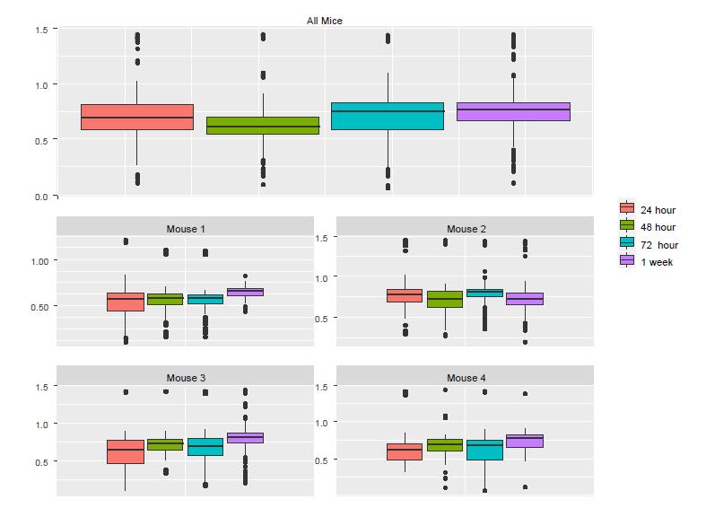
Figure S2: The boxplots of Ca++ event frequencies measured at four time points. (A) Boxplot of Ca++ event
frequencies using the pooled neurons from four mice. (B) boxplots of Ca++ event frequencies stratified by
individual mice.
To examine why the pooled data follow the pattern of Mouse 2 and not that of other mice, we checked the number of neurons in each of the mouse-by-time combinations.
# one mouse contributed 43% cells
# the number of cells in each animal-time combination
table(Ex2$midx, Ex2$treatment_idx)
# compute the percent of cells contributed by each mouse
rowSums(table(Ex2$midx, Ex2$treatment_idx))/1724
| 24h | 48h | 72h | 1wk | Total | |
| Mouse 1 | 81 | 254 | 88 | 43 | 466 (27%) |
| Mouse 2 | 206 | 101 | 210 | 222 | 739 (43%) |
| Mouse 3 | 33 | 18 | 51 | 207 | 309 (18%) |
| Mouse 4 | 63 | 52 | 58 | 37 | 210 (12%) |
| Total | 383 | 425 | 407 | 509 | 1,724 (100%) |
The last column of the table above shows that Mouse 2 contributed 43% cells, which likely explains why the pooled data are more similar to Mouse 2 than to the other mice. The lesson from this example is that naively pooling data from different animals is a potentially dangerous practice, as the
results can be dominated by a single animal that can misrepresent the data. Application of LME solves this troubling potential problem as it takes dependency and weighting into account.
In this example, the number of levels in the random-effects variable is four, as there are four mice. This number may be smaller than the recommended number for using random-effects. However, as discussed in Gelman and Hill (2007), using a random-effects model in this situation of a small sample size might not do much harm. An alternative is to include the animal ID variable as a factor with fixed animal effects in the conventional linear regression. Note that neither of the two analyses is the same as fitting a linear model to the pooled cells together, which erroneously ignores the between-animal heterogeneity and fails to account for the data dependency due to the within-animal similarity. In a more extreme case, for an experiment using only two monkeys for example, naively pooling the neurons from the two animals faces the risk of making conclusions mainly from one animal and unrealistic homogeneous assumptions across animals, as discussed above. A more appropriate approach is to analyze the animals separately and check whether the results from these two animals “replicate” each other. Exploratory analysis such
as data visualization is highly recommended to identify potential issues.
Example 3. In this experiment, Ca++ event integrated amplitudes are compared between baseline and 24h after ketamine treatment. 622 cells were sampled from 11 mice and each cell was measured twice (baseline and after ketamine treatment). As a result, correlation arises from both cells and animals, which creates a three-level structure: measurements within cells and cells within animals. It is clear that the ketamine treatment should be treated as a fixed effect. The choice for random effects deserves more careful consideration. The hierarchical structure, i.e., two observations per cell and multiple cells per animal suggests that the random effects of cells should be nested within individual mice. By including the cell variable in the random effect, we implicitly use the change from “before” to “after” treatment for each cell. This is similar to how paired data are handled in a paired t-test. Moreover, by specifying that the cells are nested within individual mice, we essentially model the correlations at both mouse and cell levels.
> Ex3=read.csv("Example3.txt", head=T)
>
> #### wrong analysis: using the linear model
> summary(lm(res~treatment, data=Ex3[!is.na(Ex3$res),])) #0.0036
Call:
lm(formula = res ~ treatment, data = Ex3[!is.na(Ex3$res), ])
Residuals:
Min 1Q Median 3Q Max
-3.1311 -1.3203 -0.1806 1.1438 6.7518
Coefficients:
Estimate Std. Error t value Pr(>|t|)
(Intercept) 2.73206 0.10817 25.258 <2e-16 ***
treatment 0.19952 0.06847 2.914 0.0036 **
---
Signif. codes: 0 ‘***’ 0.001 ‘**’ 0.01 ‘*’ 0.05 ‘.’ 0.1 ‘ ’ 1
Residual standard error: 1.708 on 2487 degrees of freedom
Multiple R-squared: 0.003403, Adjusted R-squared: 0.003002
F-statistic: 8.492 on 1 and 2487 DF, p-value: 0.0036
> #### wrong anlaysis using t tests (paired or unpaired)
> t.test(Ex3[Ex3$treatment==1,"res"], Ex3[Ex3$treatment==2,"res"], var.eq=T)
> t.test(Ex3[Ex3$treatment==1,"res"], Ex3[Ex3$treatment==2,"res"])
> t.test(Ex3[Ex3$treatment==1,"res"], Ex3[Ex3$treatment==2,"res"], paired=T)
>#correct analysis
> lme.obj=lme(res~ treatment, random =~1| midx/cidx, data= Ex3[!is.na(Ex3$res),] ,
method="ML")
> summary(lme.obj)
Linear mixed-effects model fit by maximum likelihood
Data: Ex3[!is.na(Ex3$res), ]
AIC BIC logLik
9378.498 9407.596 -4684.249
Random effects:
Formula: ~1 | midx
S18
(Intercept)
StdDev: 0.404508
Formula: ~1 | cidx %in% midx
(Intercept) Residual
StdDev: 1.083418 1.259769
Fixed effects: res ~ treatment
Value Std.Error DF t-value p-value
(Intercept) 2.7983541 0.15017647 1240 18.633772 0e+00
treatment 0.1934755 0.05055295 1240 3.827184 1e-04
Correlation:
(Intr)
treatment -0.504
Standardized Within-Group Residuals:
Min Q1 Med Q3 Max
-2.69833206 -0.60733714 -0.09362515 0.52748499 3.91394332
Number of Observations: 2489
Number of Groups:
midx cidx %in% midx
11 1248
For the treatment effect, LME and LM produce similar estimates; however, the standard error of the LM is larger. As a result, the p-value based on LME is smaller (0.0036 for LM vs 0.0001 for LME). In this example, since the two measures from each cell are positively correlated, as shown in the Figure S3, the variance of the differences is smaller when treating the data as paired rather than independent. As a result, LME produces a smaller p-value than the t-test. As a result, the more rigorous practice of using cell effects as random effects leads to a lower p-value for Example 3.
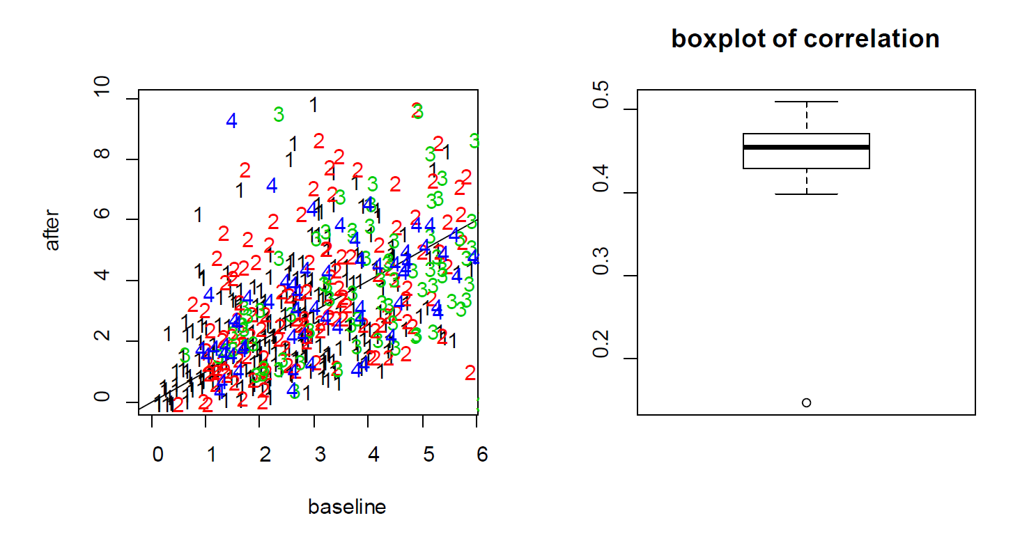
the neurons from four mice (labeled as 1, 2, 3 and 4) indicates that the baseline and after-treatment
measures are positively correlated. (Right) boxplot of the baseline and after-treatment correlations of the
11 mice.
A note on “nested” random effects. When specifying the nested random effects, we used “random =~1| midx/cidx”. This leads to random effects at two levels: the mouse level and the cells-within-mouse level. This specification is important if same cell IDs might appear in different mice. When each cell has its unique ID, just like “cidx” variable in Example 3, it does not matter and “random =list(midx=~1, cidx=~1)” leads to exactly the same model.
### to verify that the cell IDs are indeed unique
> length(unique(Ex3$cidx))
[1] 1248
#lme.obj2 is the same as lme.obj
> lme.obj2=lme(res~ treatment, random =list(midx=~1, cidx=~1), data=
Ex3[!is.na(Ex3$res),] , method="ML")
> summary(lme.obj2)
Linear mixed-effects model fit by maximum likelihood
Data: Ex3[!is.na(Ex3$res), ]
AIC BIC logLik
9378.498 9407.596 -4684.249
Random effects:
Formula: ~1 | midx
(Intercept)
StdDev: 0.404508
Formula: ~1 | cidx %in% midx
(Intercept) Residual
StdDev: 1.083418 1.259769
Fixed effects: res ~ treatment
Value Std.Error DF t-value p-value
(Intercept) 2.7983541 0.15017647 1240 18.633772 0e+00
treatment 0.1934755 0.05055295 1240 3.827184 1e-04
Correlation:
(Intr)
treatment -0.504
Standardized Within-Group Residuals:
Min Q1 Med Q3 Max
-2.69833206 -0.60733714 -0.09362515 0.52748499 3.91394332
Number of Observations: 2489
Number of Groups:
midx cidx %in% midx
11 1248
On models with more random effects. The above LME model only involves random intercepts. When there are random effects due to multiple sources, it is often recommended to fit a large model (in the sense of as many random effects as possible) to avoid obtaining false positives. However, studies also find that fitting the maximal model can cause decreased statistical power. Visualization is a useful exploratory tool to help identify an appropriate model. Figure S4 shows two common ways to visualize data in an exploratory data analysis: the scatter plots and the so-called “spaghetti” plots. The spaghetti plots indicate that neurons are quite different from each other in terms of both baseline values and
changes; the scatter plots with linear model fit suggest that the animals are different from each other at least at the starting baseline. Together, they suggest that random slopes are needed at least at the neuron level.
Here we consider three alternative models (lme.obj3, lme.obj4, lme.obj5) that include additional random effects. More specifically, lme.obj3 includes random slopes only at the neuron level; lme.obj4 includes random slopes only at the animal level; and lme.obj5 includes random slopes for both neurons and animals.
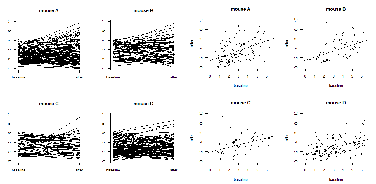
mice (labeled as A, B, C and D) with each dot representing a neuron. The four plots on the left are
“spaghetti” plots of the four animals with each line representing the values at baseline and 24h after
treatment for a neuron; the four plots on the right report the before-after scatter plots (with fitted straight
lines using a simple linear regression).
> #mouse: random intercepts; neuron: both random intercepts and random slopes
> #(independence not assumed)
> lme.obj3=lme(res~ treatment, random=list(midx=~1, cidx=~treatment), data=
Ex3[!is.na(Ex3$res),], method="ML")
> summary(lme.obj3)
Linear mixed-effects model fit by maximum likelihood
Data: Ex3[!is.na(Ex3$res), ]
AIC BIC logLik
9272.45 9313.187 -4629.225
Random effects:
Formula: ~1 | midx
(Intercept)
StdDev: 0.4302823
Formula: ~treatment | cidx %in% midx
Structure: General positive-definite, Log-Cholesky parametrization
StdDev Corr
(Intercept) 1.529776 (Intr)
treatment 1.159775 -0.724
Residual 0.956257
Fixed effects: res ~ treatment
Value Std.Error DF t-value p-value
(Intercept) 2.808037 0.15076357 1240 18.625434 0e+00
treatment 0.191860 0.05057672 1240 3.793445 2e-04
Correlation:
(Intr)
treatment -0.425
Standardized Within-Group Residuals:
Min Q1 Med Q3 Max
-2.26228406 -0.47042693 -0.07585988 0.42870152 2.37367673
Number of Observations: 2489
Number of Groups:
midx cidx %in% midx
11 1248
> anova(lme.obj1, lme.obj3)
Model df AIC BIC logLik Test L.Ratio p-value
lme.obj1 1 5 9378.498 9407.596 -4684.249
lme.obj3 2 7 9272.450 9313.187 -4629.225 1 vs 2 110.0484 <.0001
>
> #mouse: random intercepts and random slopes (independence not assumed); neuron:
random intercepts
> lme.obj4=lme(res~ treatment, random=list(midx=~treatment, cidx=~1), data=
Ex3[!is.na(Ex3$res),], method="ML")
> summary(lme.obj4)
Linear mixed-effects model fit by maximum likelihood
Data: Ex3[!is.na(Ex3$res), ]
AIC BIC logLik
9379.713 9420.451 -4682.857
Random effects:
Formula: ~treatment | midx
Structure: General positive-definite, Log-Cholesky parametrization
StdDev Corr
(Intercept) 0.5482023 (Intr)
treatment 0.1393209 -0.784
Formula: ~1 | cidx %in% midx
(Intercept) Residual
StdDev: 1.085417 1.256165
Fixed effects: res ~ treatment
Value Std.Error DF t-value p-value
(Intercept) 2.822533 0.18848581 1240 14.97477 0.0000
treatment 0.178527 0.06703098 1240 2.66335 0.0078
Correlation:
(Intr)
treatment -0.758
Standardized Within-Group Residuals:
Min Q1 Med Q3 Max
-2.6551618 -0.6096016 -0.0860911 0.5312087 3.8846466
Number of Observations: 2489
Number of Groups:
midx cidx %in% midx
11 1248
> #mouse: random intercepts and random slopes; neuron: random intercepts and random
slopes
> lme.obj5=lme(res~ treatment, random= ~ 1+treatment | midx/cidx, data=
Ex3[!is.na(Ex3$res),], method="ML")
> summary(lme.obj5)
Linear mixed-effects model fit by maximum likelihood
Data: Ex3[!is.na(Ex3$res), ]
AIC BIC logLik
9272.72 9325.097 -4627.36
Random effects:
Formula: ~1 + treatment | midx
Structure: General positive-definite, Log-Cholesky parametrization
StdDev Corr
(Intercept) 0.5727292 (Intr)
treatment 0.1423942 -0.84
Formula: ~1 + treatment | cidx %in% midx
Structure: General positive-definite, Log-Cholesky parametrization
StdDev Corr
(Intercept) 1.5670930 (Intr)
treatment 1.1781355 -0.731
Residual 0.9400533
Fixed effects: res ~ treatment
Value Std.Error DF t-value p-value
(Intercept) 2.8318145 0.18997195 1240 14.906488 0.0000
treatment 0.1745063 0.06743067 1240 2.587937 0.0098
Correlation:
(Intr)
treatment -0.758
Standardized Within-Group Residuals:
Min Q1 Med Q3 Max
-2.24686402 -0.46954860 -0.07119766 0.42205349 2.36058720
Number of Observations: 2489
Number of Groups:
midx cidx %in% midx
11 1248
> anova(lme.obj1, lme.obj3)
Model df AIC BIC logLik Test L.Ratio p-value
lme.obj1 1 5 9378.498 9407.596 -4684.249
lme.obj3 2 7 9272.450 9313.187 -4629.225 1 vs 2 110.0484 <.0001
> anova(lme.obj1, lme.obj4)
Model df AIC BIC logLik Test L.Ratio p-value
lme.obj1 1 5 9378.498 9407.596 -4684.249
lme.obj4 2 7 9379.713 9420.451 -4682.857 1 vs 2 2.784563 0.2485
> anova(lme.obj3, lme.obj5)
Model df AIC BIC logLik Test L.Ratio p-value
lme.obj3 1 7 9272.45 9313.187 -4629.225
lme.obj5 2 9 9272.72 9325.097 -4627.360 1 vs 2 3.729136 0.155
The comparisons indicate that lme.obj3 improves the basic model lme.obj1 substantially; the improvement brought by lme.obj4 is less impressive; and lme.obj3, the model with random intercepts and slopes at the neuron level, and random intercepts at the animal level appears adequate. This is
supported by the observable differences in baseline values and changes even for cells within the same animal (Figure S4). This suggests that including random intercepts and slopes at the neuron level is necessary.
A note on the testing of random-effects. The comparisons using the “anova” function suggests that lme.obj4, which assumes random intercepts and random slopes at the animal level and random intercepts at neuron level, might be adequate. It should be kept in mind that these comparisons based on likelihood ratio tests and the p-values are conservative. This is because these hypothesis problems are testing parameters at their boundary (Self and Liang 1987). Without getting into many details, the consequence is that the null distribution for the likelihood ratio test is no longer valid and the p-value will be overestimated. Obtaining the correct null distribution is not straightforward and requires advanced considerations beyond the scope of this article. However, (Fitzmaurice et al., 2012) suggests the ad-hoc rule to use a level of significance α=0.1, instead of the typical α =0.05, when judging the statistical significance of the likelihood ratio test. We adopted this suggestion in interpreting the results above.
It should also be noted that decisions should not be based on tests and p-values alone. Results can be significant with a very small effect size and large sample size or might not reach significance from a moderate or large effect size but based on a small sample size. Rather, these decisions should be based on study design, scientific reasoning, experience, or previous studies. For example, different animals are expected to have different mean levels on outcome variables; thus, it is reasonable to model the variation due to animals by considering animal specific effects. A similar argument is the inclusion of baseline covariates such as age in many medical studies even when they are not significant. Also, when random
slopes are included, it is typically recommended to include the corresponding random intercepts. For example, if the random slopes (for treatment) are included at the animal level, it is also sensible to include the animal-specific random intercepts.
Conduct GLMM using R.
Traditional linear models and LME should be designed to model a continuous outcome variable with a fundamental assumption that its variance does not change with its mean. This assumption is easily violated for commonly collected outcome variables, such as the choice made in a two-alternative forced choice task (binary data), the proportion of neurons activated (proportional data), the number neural spikes in a given time window, and the number of behavioral freezes in each session (count data). These types of outcome variables can be analyzed using a framework called generalized linear models, which are further extended to generalized linear mixed-effects models (GLMM) for correlated data. The computation involved in GLMM is more much challenging. The “glmer” function in the lme4 package can be used to fit a GLMM, which will be shown in Example 4.
Example 4. In the previous examples, the outcomes of interest are continuous. In particular, some were transformed from original measures so that the distribution of the outcome variable still has a rough bell shape. In many situations, the outcome variable we are interested has a distribution that far away from normal. Consider a simulated data set based upon part of the data used in Wei et al 2020. In our simulated data, a tactile delayed response task, eight mice were trained to use their whiskers to predict the location (left or right) of a water pole and report it with directional licking (lick left or lick right). The behavioral outcome we are interested in is whether the animals made the correct predictions.
Therefore, we code correct left or right licks as 1 and erroneous licks as 0. In total, 512 trials were generated, which include 216 correct trials and 296 wrong trials. One question we would like to answer is whether a particular neuron is associated with the prediction. For that purpose, we analyze the prediction outcome and mean neural activity levels (measured by dF/F) from the 512 trials using a GLMM. The importance of modeling correlated data by introducing random effects has been shown in the previous examples. In this example, we focus on how to interpret results from a GLMM model in the water lick experiment.
Like a GLM, a GLMM requires the specification of a family of the distributions of the outcomes and an appropriate link function. Because the outcomes in this example are binary, the natural choice, which is often called the canonical link of the “binomial” family, is the logistic link. For each family of distributions, there is a canonical link, which is well defined and natural to that distribution family. For researchers with limited experience with GLM or GLMM, a good starting point, which is often a reasonable choice, is to use the default choice (i.e., the canonical link).
library(lme4) #the main functions are "lmer" and glmer
library(pbkrtest)
#read data from the file named “waterlick_sim.txt”
waterlick=read.table("waterlick_sim.txt", head=T)
#take a look at the data
summary(waterlick)
#change the mouseID to a factor
waterlick[,1]=as.factor(waterlick[,1])
#use glmer to fit a GLMM model
obj.glmm=glmer(lick~dff+(1|mouseID),
data=waterlick,family="binomial")
#summarize the model
> summary(obj.glmm)
Generalized linear mixed model fit by maximum likelihood (Laplace Approximation)
[glmerMod
]
Family: binomial ( logit )
Formula: lick ~ dff + (1 | mouseID)
Data: waterlick
AIC BIC logLik deviance df.resid
679.8 692.5 -336.9 673.8 509
Scaled residuals:
Min 1Q Median 3Q Max
-1.4854 -0.8375 -0.6196 1.0265 1.9641
Random effects:
Groups Name Variance Std.Dev.
mouseID (Intercept) 0.106 0.3255
Number of obs: 512, groups: mouseID, 8
Fixed effects:
Estimate Std. Error z value Pr(>|z|)
(Intercept) -0.63382 0.17753 -3.570 0.000357 ***
dff 0.06235 0.01986 3.139 0.001693 **
---
Signif. codes: 0 ‘***’ 0.001 ‘**’ 0.01 ‘*’ 0.05 ‘.’ 0.1 ‘ ’ 1
Correlation of Fixed Effects:
(Intr)
dff -0.550
#compute increase in odds and a 95% CI
> exp(c(0.06235, 0.06235-1.96*0.01986, 0.06235+1.96*0.01986))-1
[1] 0.06433480 0.02370091 0.10658157
The default method of parameter estimation is the maximum likelihood with Laplace approximation. As shown in the Fixed effects section of the R output, the estimated increase in log-odds associated with one percent increase in dF/F is 0.06235 with a standard error of 0.01986 and the p-value
(which is based on the large-sample Wald test) is 0.01693. Correspondingly, an approximate 95% CI is (0.06235-1.96*0.01986, 0.06235+1.96*0.01986), i.e., (0.0234244 0.1012756). In a logistic regression, the estimated coefficient of an independent variable is typically interpreted using the percentage of odds changed for a one-unit increase in the independent variable. In this example, exp(0.06235)=1.064,
indicating that the odds of making correct licks increased by 6.4% (95% C.I.: 2.4%-10.7%) with one percent increase in dF/F.
An alternative way to compute a p-value is to use a likelihood ratio test by comparing the likelihoods of the current model and a reduced model.
#fit a smaller model, the model with the dff variable removed
obj.glmm.smaller=glmer(lick~(1|mouseID),

data=waterlick,family="binomial")
#use the anova function to compare the likelihoods of the two models
> anova(obj.glmm, obj.glmm.smaller)
Data: waterlick
Models:
obj.glmm.smaller: lick ~ (1 | mouseID)
obj.glmm: lick ~ dff + (1 | mouseID)
npar AIC BIC logLik deviance Chisq Df Pr(>Chisq)
obj.glmm.smaller 2 687.77 696.24 -341.88 683.77
obj.glmm 3 679.77 692.48 -336.88 673.77 9.9964 1 0.001568 **
---
Signif. codes: 0 ‘***’ 0.001 ‘**’ 0.01 ‘*’ 0.05 ‘.’ 0.1 ‘ ’ 1
#alternatively, one can use the “drop1” function to test the effect of dfff
> drop1(obj.glmm, test="Chisq")
Single term deletions
Model:
lick ~ dff + (1 | mouseID)
npar AIC LRT Pr(Chi)
<none> 679.77
dff 1 687.77 9.9964 0.001568 **
---
Signif. codes: 0 ‘***’ 0.001 ‘**’ 0.01 ‘*’ 0.05 ‘.’ 0.1 ‘ ’ 1
In the output from “anova(obj.glmm, obj.glmm.smaller)”, the “Chisq” is the -2*log(L0/L1), where L1 is the maximized likelihood of the model with dff and L0 is the maximized likelihood of the model without the dff. The p-value was obtained using the large-sample likelihood ratio test.
In GLMM, the p-value based on large-sample approximations might not be accurate. It is helpful to check whether nonparametric tests lead to similar findings. For example, one can use a parametric bootstrap method. For this example, the p-value from the parametric bootstrap test, which is slightly less significant than the p-values from the Wald or LRT test.
> PBmodcomp(obj.glmm, obj.glmm.smaller)
Bootstrap test; time: 333.45 sec;samples: 1000; extremes: 0;
Requested samples: 1000 Used samples: 999 Extremes: 0
large : lick ~ dff + (1 | mouseID)
small : lick ~ (1 | mouseID)
stat df p.value
LRT 9.9964 1 0.001568 **
PBtest 9.9964 0.001000 ***
---
Signif. codes: 0 ‘***’ 0.001 ‘**’ 0.01 ‘*’ 0.05 ‘.’ 0.1 ‘ ’ 1
There were 16 warnings (use warnings() to see them)
By default, 1000 samples were generated to understand the null distribution of the likelihood ratio statistic. When a p-value is small, 1000 samples might not return an accurate estimation. In this situation, one can increase the number of samples to 10,000 or even more. One way to expedite
computation is by using multiple cores. We encourage the interested readers to read the documentation of this package, which is available at https://cran.rproject.org/web/packages/pbkrtest/pbkrtest.pdf.
A note on convergence. Compared to LME, GLMM is harder to converge. When increasing the number of iterations does not work, one can change the likelihood approximation methods and numerical maximization methods. If convergence is still problematic, one might want to consider modifying models. For example, eliminating some random effects will likely make the algorithm converge. In particular, when the number of levels of a categorical variable is small, using fixed- rather than random- effects might help resolve the convergence issues. Using Bayesian alternatives might also be helpful. We recommend readers to check several relevant websites for further guidance:
https://rstudio-pubs-static.s3.amazonaws.com/33653_57fc7b8e5d484c909b615d8633c01d51.html
https://bbolker.github.io/mixedmodels-misc/glmmFAQ.html
https://m-clark.github.io/posts/2020-03-16-convergence/
A Bayesian Analysis of Example 4. In the LME and GLMM framework, the random effect coefficients are assumed as being drawn from a given distribution. Therefore, Bayesian analysis provides a natural alternative for analyzing multilevel/ hierarchical data. Statistical inference in Bayesian analysis is from the posterior distribution of the parameters, which is proportional to the product of the likelihood of the data and the prior distribution of the parameters. Here we use the “brms” package to analyze the water lick data. The package performs Bayesian regression in multilevel models using the software “Stan” for full Bayesian (Bürkner, 2017; Bürkner, 2018). Due to the lack of prior information, we select priors that are relatively non-informative, i.e., have large variances around their mean. More specifically, we use a normal prior with mean 0 and large standard deviation 10 for the fixed-effect coefficients. For the variances of the random intercept and the errors, we assume a half-Cauchy distribution with a scale parameter of 5.
library(brms)#it might ask you to install other necessary packages
waterlick=read.table("waterlick_sim.txt", head=T)
obj.brms=brm(formula = lick ~ dff + (1|mouseID),
data=waterlick, family="bernoulli",
prior = c( set_prior("normal(0,10)", class="b"),
set_prior("cauchy(0,5)", class="sd")),warmup=1000, iter=2000, chains=4,control = list(adapt_delta = 0.95), save_all_pars = TRUE)
> summary(obj.brms)
Family: bernoulli
Links: mu = logit
Formula: lick ~ dff + (1 | mouseID)
Data: waterlick (Number of observations: 512)
Samples: 4 chains, each with iter = 2000; warmup = 1000; thin = 1;
total post-warmup samples = 4000
Group-Level Effects:
~mouseID (Number of levels: 8)
Estimate Est.Error l-95% CI u-95% CI Rhat Bulk_ESS Tail_ESS
sd(Intercept) 0.46 0.23 0.08 1.02 1.01 765 732
Population-Level Effects:
Estimate Est.Error l-95% CI u-95% CI Rhat Bulk_ESS Tail_ESS
Intercept -0.63 0.23 -1.08 -0.14 1.01 1305 1803
dff 0.06 0.02 0.02 0.10 1.00 2780 2616
Samples were drawn using sampling(NUTS). For each parameter, Bulk_ESS
and Tail_ESS are effective sample size measures, and Rhat is the potential
scale reduction factor on split chains (at convergence, Rhat = 1).
> summary(obj.brms)$fixed
Estimate Est.Error l-95% CI u-95% CI Rhat Bulk_ESS Tail_ESS
Intercept -0.62627973 0.23101575 -1.08084815 -0.1373140 1.005906 1305 1803
dff 0.06105309 0.02058415 0.02182994 0.1026825 1.000328 2780 2616
The results show that the odds that the mice will make a correct prediction increase by 6.2% (95% credible interval: 2.0%-10.6%) with 1% increase in dF/F. The use of a Bayesian approach and the Bayes factors have been advocated as an alternative to p-values since the Bayes factor represents a direct measure of the evidence of one model versus the other. Typically, it is recognized that a Bayes Factor greater than 150 provides a very strong evidence of a hypothesis, say H1, against another hypothesis, say H0; a Bayes Factor between 20 and 150 provides strong evidence of the plausibility of H1, whereas if the Bayes Factor is between 3 and 20, it provides only positive evidence for H1. A value of the Bayes Factor between 1 and 3 is not worth more than a bare mention (Held and Ott, 2018; Kass and Raftery, 1995). In the following computation, we find that the Bayes factor of the model with dF/F versus the null model is 5.02, suggesting moderate association of dF/F with correct licks. These results are comparable to those from the frequentist GLMM in the previous paragraph.
#Note: to compute a Bayes factor, we need to use “save_all_pars=TRUE” option
#the reduced model is
obj0.brms=brm(formula = lick ~ 1+ (1|mouseID),
data=waterlick, family="bernoulli",
prior = c(set_prior("cauchy(0,5)", class="sd")),
warmup=1000, iter=2000, chains=4,
control = list(adapt_delta = 0.95),save_all_pars = TRUE)
> summary(obj0.brms)
Family: bernoulli
Links: mu = logit
Formula: lick ~ 1 + (1 | mouseID)
Data: waterlick (Number of observations: 512)
Samples: 4 chains, each with iter = 2000; warmup = 1000; thin = 1;
total post-warmup samples = 4000
Group-Level Effects:
~mouseID (Number of levels: 8)
Estimate Est.Error l-95% CI u-95% CI Rhat Bulk_ESS Tail_ESS
sd(Intercept) 0.65 0.28 0.28 1.37 1.00 745 849
Population-Level Effects:
Estimate Est.Error l-95% CI u-95% CI Rhat Bulk_ESS Tail_ESS
Intercept -0.34 0.26 -0.85 0.17 1.00 831 1017
Samples were drawn using sampling(NUTS). For each parameter, Bulk_ESS
and Tail_ESS are effective sample size measures, and Rhat is the potential
scale reduction factor on split chains (at convergence, Rhat = 1).
#compare the two models by computing the Bayes factor: the one with dff vs the null
> bayes_factor(obj.brms, obj0.brms)
Iteration: 1
Iteration: 2
Iteration: 3
Iteration: 4
Iteration: 5
Iteration: 6
Iteration: 1
Iteration: 2
Iteration: 3
Iteration: 4
Iteration: 5
Estimated Bayes factor in favor of obj.brms over obj0.brms: 0.19960
#compare the models by computing the Bayes factor: the null vs the one with dff
#note that this Bayes factor is the reciprocal of the previous one
> bayes_factor(obj0.brms, obj.brms)
Iteration: 1
Iteration: 2
Iteration: 3
Iteration: 4
Iteration: 5
Iteration: 6
Iteration: 1
Iteration: 2
Iteration: 3
Iteration: 4
Iteration: 5
Estimated Bayes factor in favor of obj0.brms over obj.brms: 5.01865
References:
Bates, D., Mächler, M., Bolker, B., and Walker, S. (2014). Fitting linear mixed-effects models using lme4.
arXiv preprint arXiv:14065823.
Bürkner, P.-C. (2017). brms: An R package for Bayesian multilevel models using Stan. Journal of
statistical software 80, 1-28.
Bürkner, P. (2018). Advanced Bayesian Multilevel Modeling with the R Package brms. The R Journal, 10
(1), 395.
Fitzmaurice, G.M., Laird, N.M., and Ware, J.H. (2012). Applied longitudinal analysis, Vol 998 (John Wiley
& Sons).
Fox, J., and Weisberg, S. (2018). An R companion to applied regression (Sage publications).
Halekoh, U., and Højsgaard, S. (2014). A kenward-roger approximation and parametric bootstrap
methods for tests in linear mixed models–the R package pbkrtest. Journal of Statistical Software
59, 1-30.
Held, L., and Ott, M. (2018). On p-Values and Bayes Factors. Annual Review of Statistics and Its
Application, Vol 5: 5, 393-419.
Henderson, C.R., Kempthorne, O., Searle, S.R., and Von Krosigk, C. (1959). The estimation of
environmental and genetic trends from records subject to culling. Biometrics 15, 192-218.
Kass, R.E., and Raftery, A.E. (1995). Bayes factors. Journal of the american statistical association 90, 773-
795.
Kuznetsova, A., Brockhoff, P.B., and Christensen, R.H.B. (2017). lmerTest Package: Tests in Linear Mixed
Effects Models. Journal of Statistical Software 82, 1-26.
Lenth, R., Singmann, H., Love, J., Buerkner, P., and Herve, M. (2019). Estimated marginal means, aka
least-squares means. R package version 1.3. 2.
Lüdecke, D. (2018). sjPlot: Data visualization for statistics in social science. R package version 2.
Pinheiro, J., and Bates, D. (2006). Mixed-effects models in S and S-PLUS (Springer Science & Business
Media).
S32
Pinheiro, J., Bates, D., DebRoy, S., Sarkar, D., and Team, R.C. (2007). Linear and nonlinear mixed effects
models. R package version 3, 1-89.
R Development Core Team (2020). R: A language and environment for statistical computing (Vienna,
Austria: R Foundation for Statistical Computing).
Wolak, M., and Wolak, M.M. (2015). Package ‘ICC’. Facilitating estimation of the Intraclass Correlation
Coefficient. Version 2.3.0.